Visual Positioning Systems
The Expert Report
Everything required to reason about, evaluate, and build a Visual Positioning System — from camera geometry to planet-scale production deployments. Written to take a capable reader, human or AI, from zero to expert fluency in one document.
01What a VPS is — and what it replaces
A Visual Positioning System is an infrastructure-plus-algorithm stack that determines a camera's 6-DoF pose — three degrees of position (x, y, z) and three of orientation (roll, pitch, yaw) — by comparing the current camera image against a previously constructed visual model of the environment. The academic name for the online problem is visual localization or camera relocalization; "VPS" is the productized, planet-or-venue-scale version of it.
The single most important framing: a VPS is a lookup against a map, not a sensor. GPS measures signals from satellites; a VPS recognizes place. Everything about VPS engineering — coverage, freshness, storage, privacy — follows from the fact that someone must build and maintain the map before anyone can localize inside it.
Why GPS is not enough
| Property | GNSS (GPS/Galileo/GLONASS) | GNSS + RTK | Visual Positioning System |
|---|---|---|---|
| Position accuracy | 3–5 m open sky; 10–50 m in urban canyons (multipath) | 1–3 cm, but needs correction infrastructure and clear sky | Typically 10–50 cm outdoors, 5–20 cm indoors/venue-scale |
| Orientation | None (course-over-ground only while moving; compass is magnetically unreliable) | None (dual-antenna setups excepted) | Full 3-axis, commonly <1–3° error |
| Indoors / underground | No signal | No signal | Works — the map is the infrastructure |
| Vertical (which floor?) | Poor (2–3× worse than horizontal) | Good with fixed base | Inherent — pose is fully 3D |
| Time to fix | Seconds (warm) to minutes (cold) | Seconds–minutes to converge | One to a few camera frames (~0.1–1 s) |
| Failure mode | Degrades noisily | Falls back to plain GNSS | Fails where map is missing, stale, or scene is ambiguous |
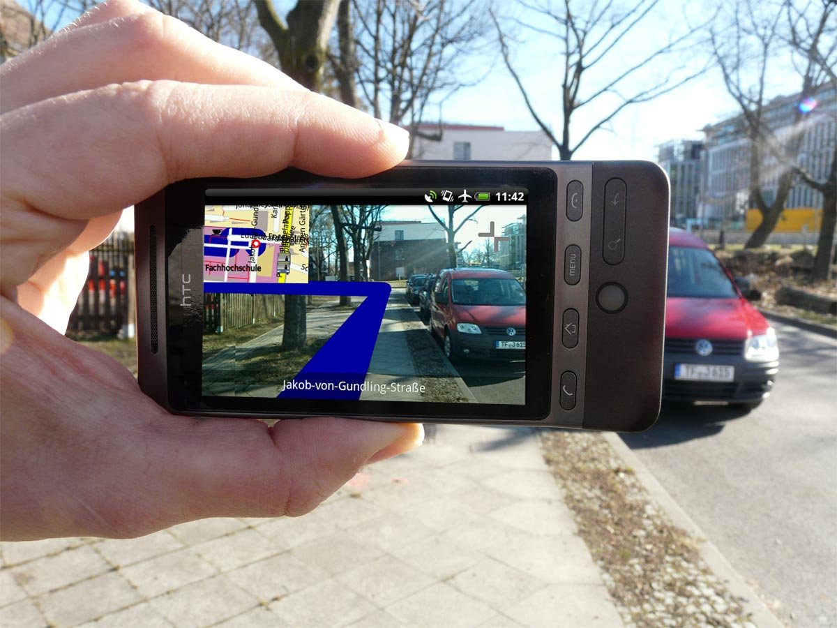
The killer capability is orientation. Augmented reality, robot manipulation, and pedestrian guidance ("the entrance is behind you") all need heading. Magnetometers drift and lie near steel; GPS heading needs motion. A VPS delivers position and a gravity-consistent, drift-free orientation from a single glance at the world.
Relatives and non-relatives
- SLAM (Simultaneous Localization and Mapping) builds a map while tracking in unknown space. A VPS localizes against a map that already exists. Production stacks use both: SLAM/VIO for smooth local tracking, VPS for absolute global anchoring (Section 8).
- Place recognition / image retrieval answers "which place is this?" (coarse, image-level). A VPS goes further to metric pose. Retrieval is the first stage of most VPS pipelines (Section 5).
- Fiducial markers (QR, AprilTag, ArUco) are the poor man's VPS: engineered features with known pose. Cheap, robust, ugly, and require physically instrumenting the space.
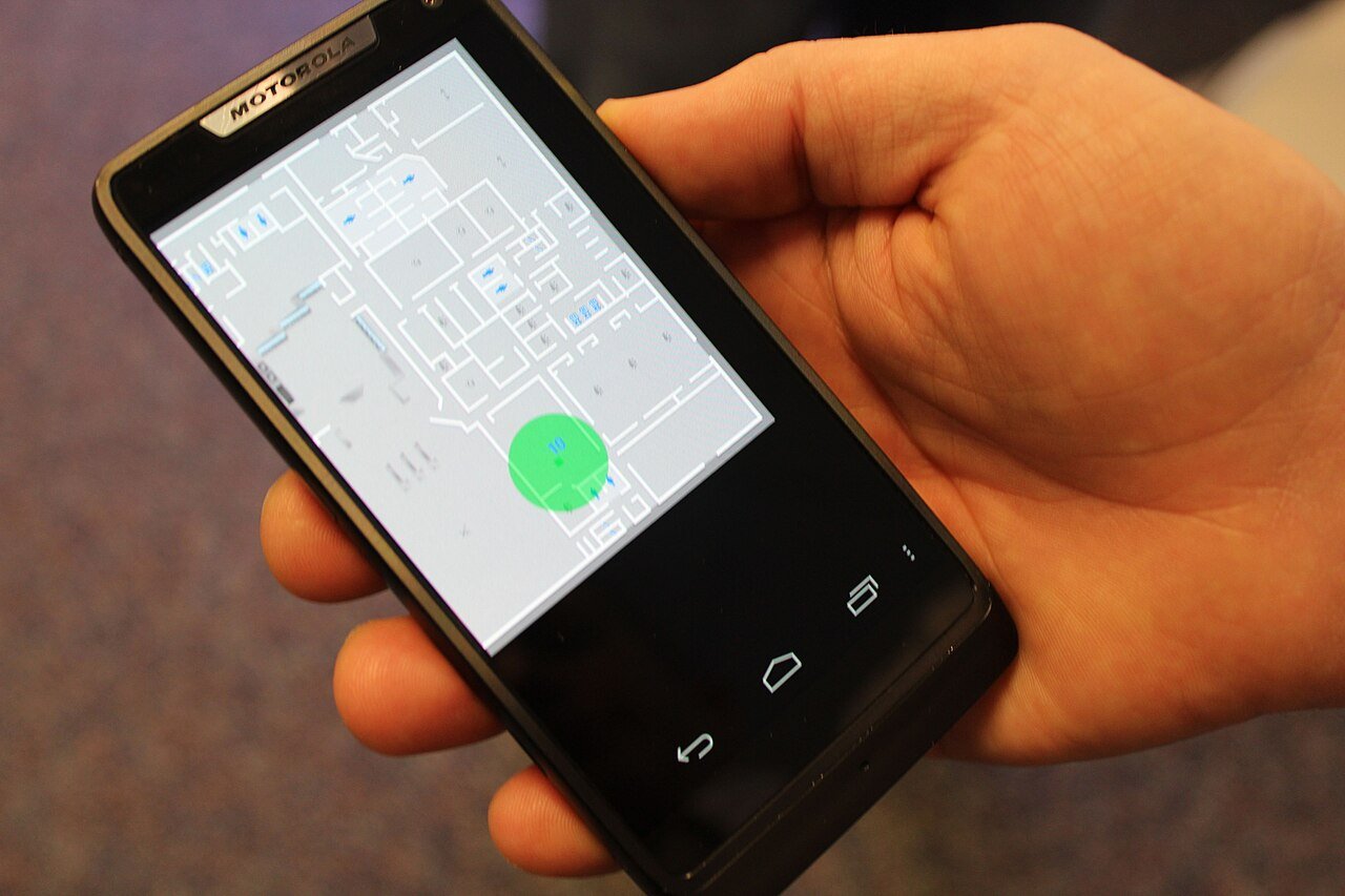
- WiFi RTT / BLE beacons / UWB give 1–5 m (WiFi/BLE) or 10–30 cm (UWB) indoor position but no orientation and require deployed radio hardware. UWB is the strongest non-visual competitor for instrumented venues.
The radio cousin — WiFi CSI (Channel State Information)
Every modern WiFi packet crosses a room as an OFDM waveform on dozens-to-thousands of subcarriers per antenna pair. To equalize the link, the receiver estimates the complex channel response — amplitude and phase, per subcarrier. That estimate, the CSI, is a multipath fingerprint of the space: every wall, cabinet, and human body contributes reflections, and any movement reshapes the response packet by packet. Read CSI as a time series and the access point becomes a passive sensor.
- Device-free sensing. Presence and intrusion detection, gesture recognition, fall detection, gait identification, even respiration monitoring — through walls, in darkness, with nothing worn or carried. The tagline is literal: the router can see you move.
- Positioning. CSI fingerprinting reaches decimeter-to-meter accuracy indoors — far beyond coarse RSSI — and time/angle-of-flight methods (WiFi RTT / 802.11mc, MIMO phase) solve position directly. Still no orientation, and still an order coarser than a VPS fix.
- Standardization and accessibility. IEEE 802.11bf is making sensing a first-class WiFi service, and ESP32 CSI toolkits put the capability on $5 microcontrollers — the hobbyist ecosystem around "ESP-CSI" is already large.
For a VPS architect, CSI is a complement, not a competitor. It is the natural upgrade to the coarse radio prior in Section 5's query package — sharper tile selection, reliable floor disambiguation — and it covers exactly the cases vision cannot: lights off, lens occluded, camera-prohibited spaces. The privacy note of Section 10 applies with extra force here: device-free sensing is consent-free by default, and it evades every camera-era intuition about when one is being watched.
02The geometric foundation
Every VPS reduces to one equation: how a 3D world point becomes a 2D pixel. Master this and the rest of the field is bookkeeping.
The pinhole projection model
- X = (X, Y, Z, 1)ᵀ — a point in the world coordinate frame (the map's frame).
- [R | t] — the extrinsics: a 3×4 matrix built from a rotation R ∈ SO(3) and translation t ∈ ℝ³ that transforms world coordinates into camera coordinates. This is the pose. This is the entire output of a VPS. The camera center in world coordinates is C = −Rᵀt — a fact interview questions love.
- K — the intrinsics: focal lengths fx, fy and principal point (cx, cy) arranged as an upper-triangular 3×3. Real lenses add radial/tangential distortion (Brown–Conrady coefficients k₁, k₂, p₁, p₂), which must be calibrated out. Phones expose calibrated intrinsics through ARKit/ARCore, which is one reason mobile VPS is tractable.
Reprojection error — the universal currency
Given a candidate pose, project every matched 3D point into the image and measure the pixel distance to where the feature was actually observed:
Reprojection error in pixels is the field's shared objective function. Mapping minimizes it over all cameras and points jointly (bundle adjustment); localization minimizes it over one camera's pose with the map fixed.
Coordinate frames — where beginners drown
A production VPS juggles at least four frames: world/map frame (often georegistered: aligned to Earth via GPS priors or surveyed control points, so poses convert to latitude/longitude/altitude + heading), camera frame, the device's VIO/odometry frame (arbitrary origin at session start, drifts over time), and gravity-aligned ENU (East-North-Up) for anything user-facing. The VPS fix is precisely the transform that pins the drifting odometry frame to the world frame. Write the frames down; most integration bugs are frame bugs, and most of those are "inverse of the transform you meant."
The PnP problem
Perspective-n-Point: given n correspondences between 3D map points and 2D pixels, plus intrinsics K, recover [R|t]. The minimal case is P3P — three correspondences give up to four solutions, disambiguated by a fourth point (geometry traceable to Grunert, 1841). EPnP solves n ≥ 4 in O(n). Standard practice: P3P inside RANSAC to find inliers and a rough pose, then Levenberg–Marquardt refinement on all inliers' reprojection error. Phones add a shortcut: the IMU gives gravity, pinning two rotational DoF, so pose search shrinks from 6-DoF to 4, making RANSAC dramatically faster and more robust.
RANSAC — trust arithmetic
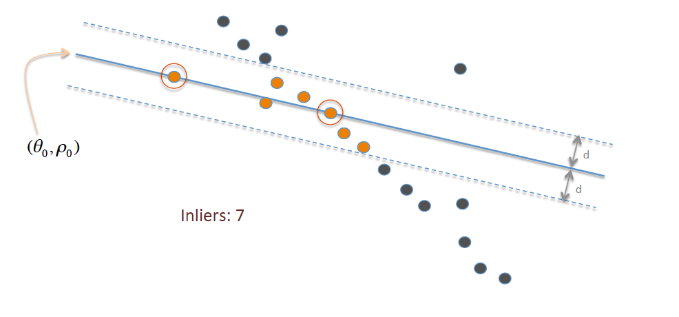
Random Sample Consensus (Fischler & Bolles, 1981 — a paper literally written about camera pose estimation): repeatedly fit a model to a minimal random sample, count how many correspondences agree within a pixel threshold, keep the best consensus set. With inlier ratio w and sample size s, the iterations needed for confidence p follow N = log(1−p)/log(1−wˢ) — which is why s matters so much: P3P's s=3 tolerates far dirtier match sets than any larger minimal problem. Modern variants (LO-RANSAC, MAGSAC++, PROSAC) refine locally, marginalize the threshold, and exploit match-quality ordering. The one-line summary an expert carries: matching proposes, RANSAC disposes.
03The two-phase architecture
Every serious VPS — Google's, Niantic's, and the one you could build with open source this weekend — has the same shape: an offline mapping pipeline that turns imagery into a localizable 3D model, and an online localization service that turns one query image into a pose in a few hundred milliseconds.
Why the hierarchy (retrieval first, matching second)? A city-scale map holds hundreds of millions of 3D points; matching a query against all of them is both intractable and self-defeating — with that many candidates, wrong-but-plausible matches swamp RANSAC (perceptual aliasing). Retrieval shrinks the search to a few dozen relevant map images, restoring both speed and precision. Coarse-to-fine is not an optimization; it is what makes city scale possible at all.
04Mapping — structure from motion
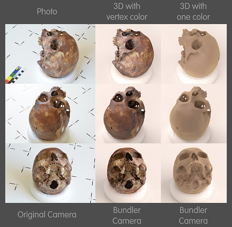
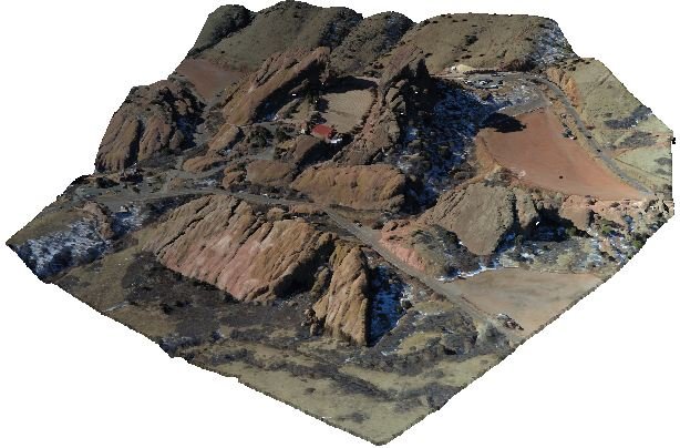
Structure from Motion (SfM) takes an unordered pile of images and recovers both the 3D structure (points) and the motion (camera poses) that produced them. The reference implementation is COLMAP (Schönberger & Frahm, 2016) — open source, battle-tested, and the substrate of most academic and many commercial pipelines.
The SfM loop
- Extract features from every image: keypoints (where) + descriptors (what it looks like). Classically SIFT; in modern pipelines a learned detector like SuperPoint (Section 6).
- Match pairs of images. Exhaustive for small sets; for large sets, retrieval or GPS priors propose candidate pairs. Verify each pair geometrically with epipolar RANSAC.
- Initialize from one well-conditioned pair (wide baseline, many inliers): recover relative pose, triangulate initial points.
- Incrementally register each new image via PnP against the growing point cloud, triangulate new points, and periodically run bundle adjustment.
Bundle adjustment — the gold standard
BA is what makes SfM maps metric-grade: errors are distributed globally instead of accumulating. The Schur complement exploits the structure (points outnumber cameras 1000:1 and don't interact directly) so million-point problems solve in minutes.
Two facts that separate experts from tourists
- Monocular SfM is scale-blind. From images alone, a cathedral and its perfect 10:1 miniature are indistinguishable. Absolute scale must be injected: GPS priors on camera positions, surveyed ground-control points, known-size objects, stereo baselines, or IMU integration. Georegistration — a similarity transform (7-DoF: rotation, translation, scale) aligning the SfM frame to Earth — is what turns a reconstruction into a positioning map with lat/long/altitude output.
- The map is not the point cloud you can see. The localizable map is: 3D points plus their visual descriptors plus the covisibility graph (which points are seen together from where) plus a retrieval index of the mapping images' global descriptors. The pretty dense mesh is a byproduct; localization runs on the sparse, descriptor-bearing skeleton.
Map sources in the wild
| Source | Example | Character |
|---|---|---|
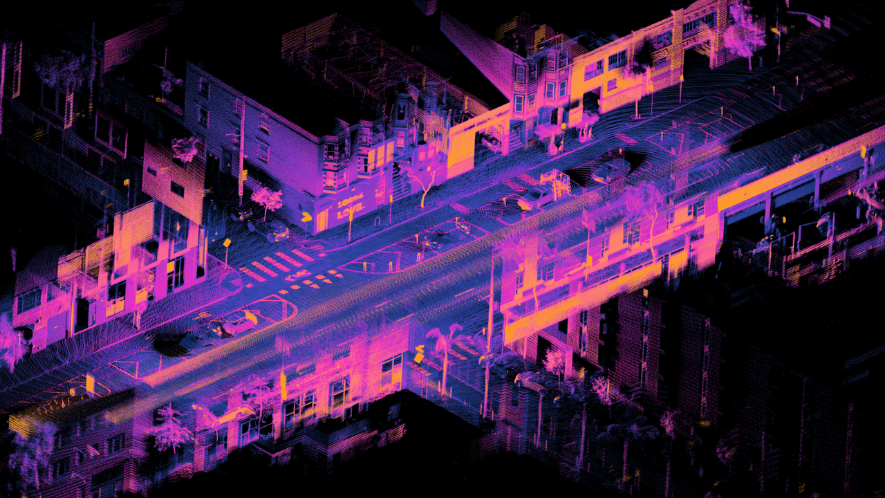
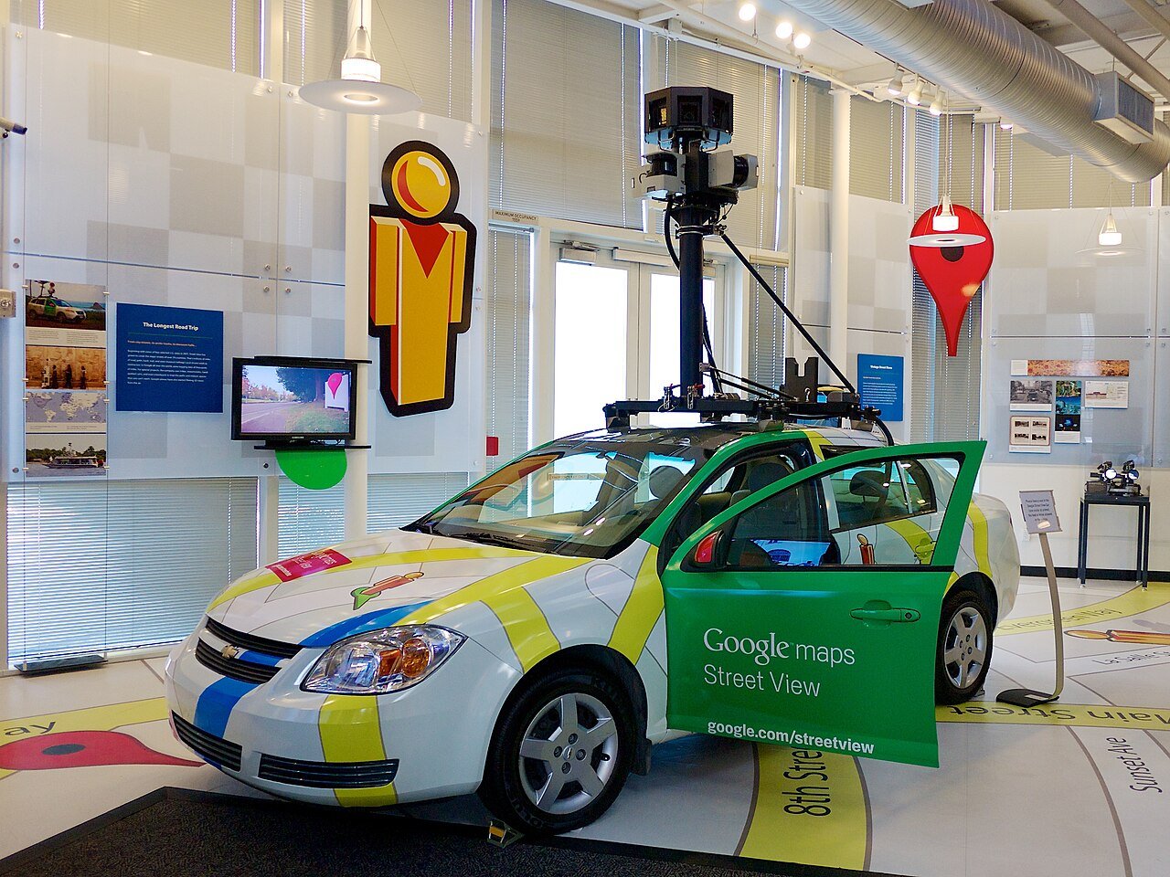
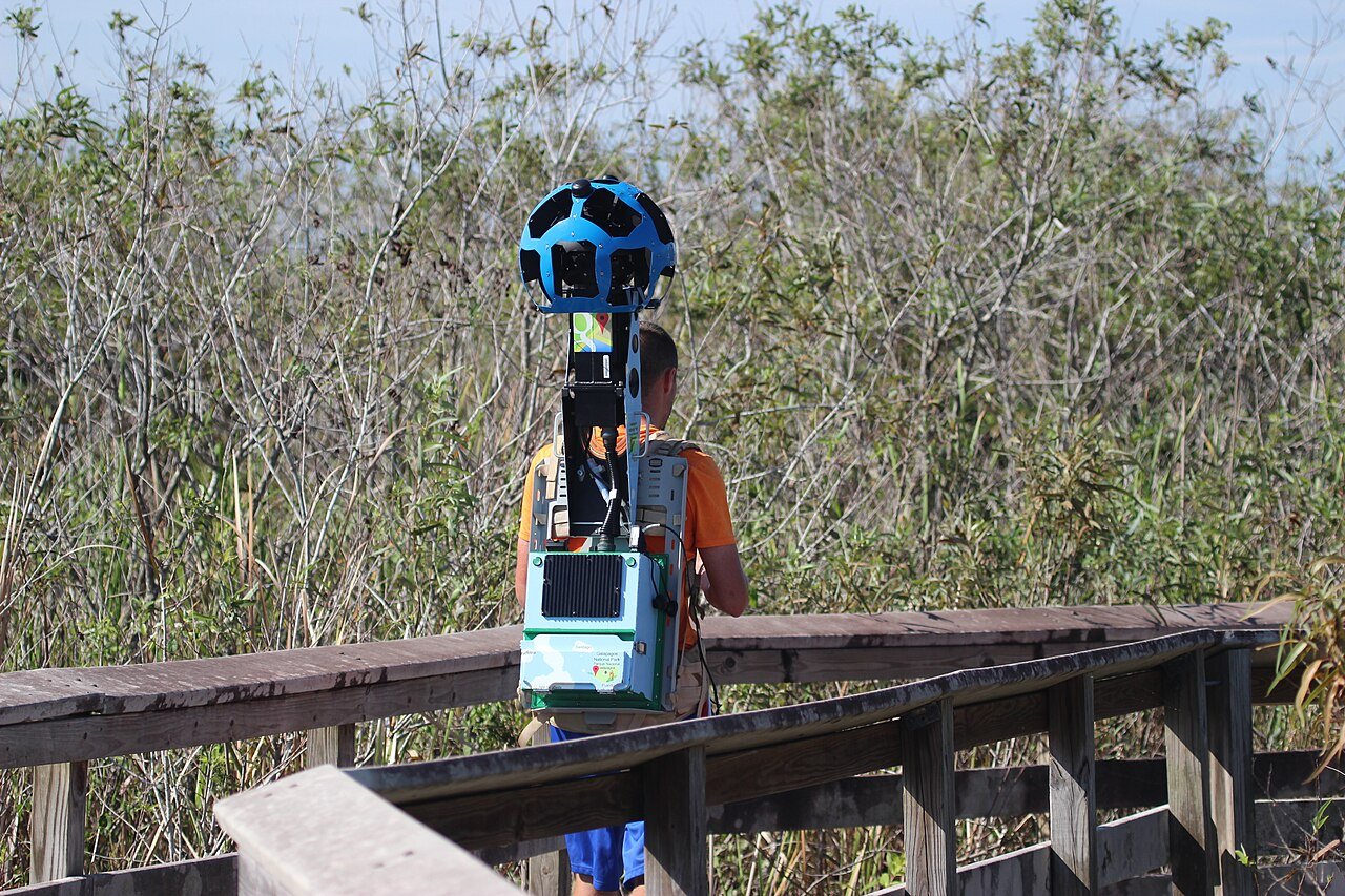
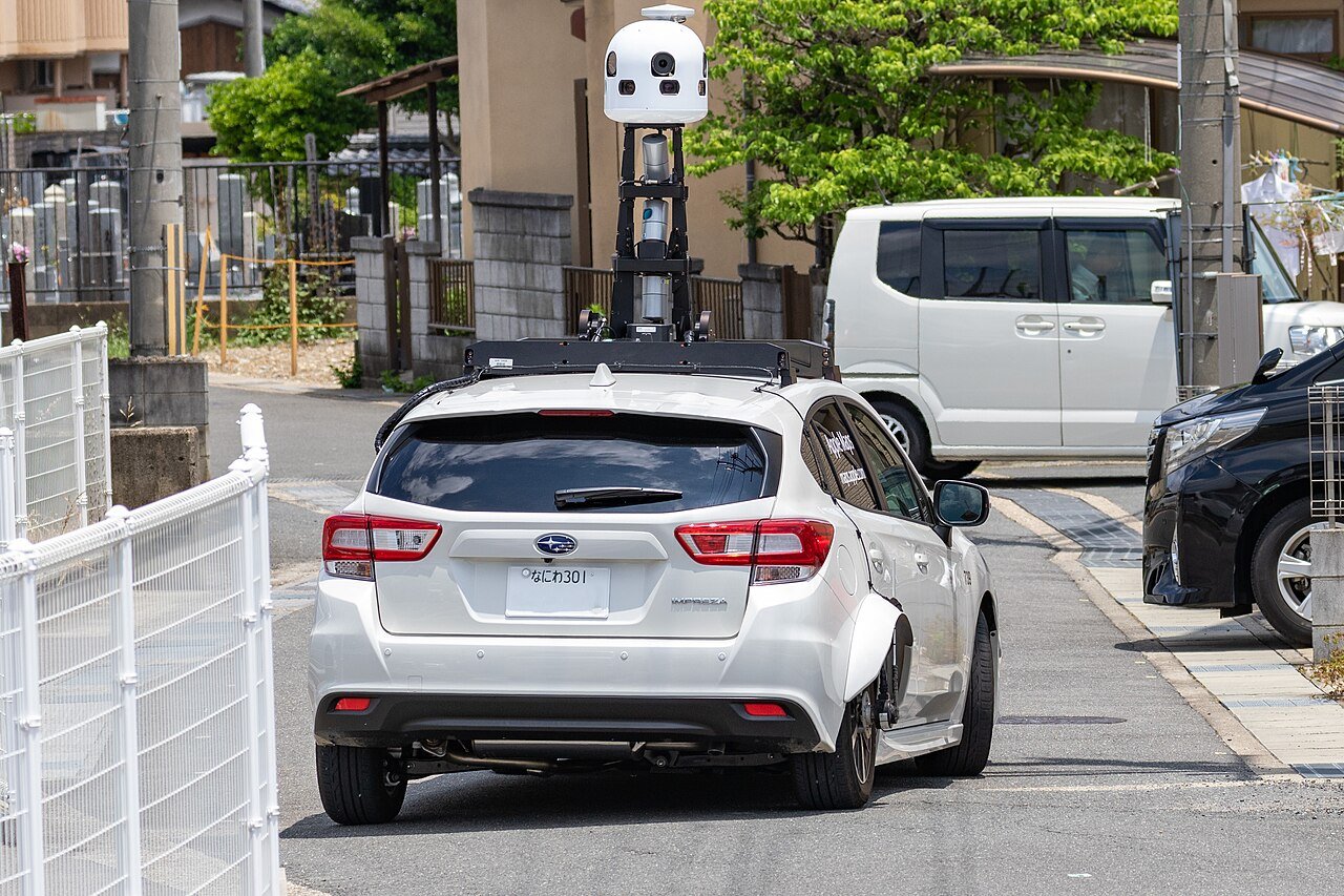
| Purpose-built survey fleets | Google Street View vehicles + Trekker rigs | Calibrated rigs, LiDAR + GPS/INS ground truth, consistent global coverage, expensive, slow refresh |
| Crowdsourced scans | Niantic (Pokémon GO / Ingress player scans, Scaniverse) | Phone-quality, massive volume, biased to points of interest, freshness for free where players go |
| Developer/venue scans | Immersal SDK, Snap Custom Landmarkers | A person walks the venue with a phone; minutes-to-hours to map; per-venue quality control |
| Existing imagery corpora | Apple Look Around; aerial/satellite for coarse layers | Reuses fleet investment; aerial-to-ground cross-view matching is an active research area |
05Localization — from one image to a pose
The online path, stage by stage, with the design choices at each:
Stage 0 — the query package
A production query is never just pixels. It carries: calibrated intrinsics (from ARKit/ARCore), gravity direction (IMU) which pins roll/pitch, a coarse position prior (GPS, cell, WiFi — selects which map tile to even consider), and often several frames rather than one. Using priors is not cheating; it is what makes planet scale feasible: GPS narrows the earth to ~100 m, retrieval narrows 100 m to ~10 images, matching narrows 10 images to one pose.
Stage 1 — image retrieval (coarse)
Encode the query into a single global descriptor vector, nearest-neighbor search against the map images' descriptors. The lineage: bag-of-visual-words and VLAD (handcrafted aggregation) → NetVLAD (2016; a CNN with a learnable VLAD pooling layer, trained on Street View time-lapse triplets — the breakthrough that made retrieval robust to day/season change) → AP-GeM, DELG → transformer/foundation-model era: AnyLoc, MixVPR, SALAD built on DINOv2 self-supervised features, which currently dominate place-recognition benchmarks. Retrieval quality gates everything downstream: if the right map images are not in the top-k, no matcher can save the query.
Stage 2 — 2D–3D correspondence (fine)
Extract local features from the query; match them against features of the retrieved map images; each map feature is tied to a triangulated 3D point, so 2D–2D matches lift to 2D–3D correspondences. Cluster retrieved images by covisibility so matches accumulate into one consistent local scene rather than several rival hypotheses.
Stage 3 — pose solving
P3P inside RANSAC (gravity-aided if available) → inlier set → Levenberg–Marquardt refinement of the pose on all inliers. Output: [R|t], inlier count, and reprojection statistics. The inlier count is the confidence signal: below a threshold (commonly a few dozen), a production system reports "no fix" rather than a guess — a wrong pose confidently delivered is far worse than none, because downstream fusion (Section 8) will propagate it.
Failure taxonomy — where queries die
| Stage | Failure | Symptom | Primary fix |
|---|---|---|---|
| Retrieval | Appearance gap (night query, day map) | Right place absent from top-k | Condition-robust global descriptors; map both conditions |
| Retrieval | Perceptual aliasing (identical corridors, chain-store facades) | Wrong-but-similar place retrieved | Position priors; geometric verification of retrieval |
| Matching | Texture-poor or repetitive surfaces | Few or structured-wrong matches | Learned matchers (context helps); denser features; lines/planes |
| PnP | Degenerate geometry (all points coplanar/distant) | Pose ambiguity, huge covariance | Multi-frame queries; report covariance honestly |
| Map | Scene changed since mapping | Consistent mismatch, low inliers everywhere | Freshness pipeline; change detection; re-map triggers |
06Features and matching — the forty-year arms race
Handcrafted era
- Harris corners (1988) — where gradients vary in two directions; detection only.
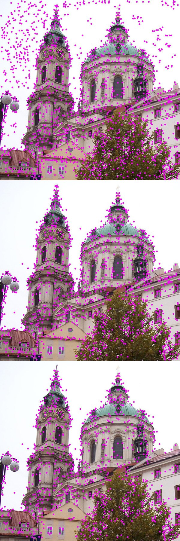
- SIFT (Lowe, 1999/2004) — the field's foundation stone: scale-space extrema detection + 128-D gradient-histogram descriptor, invariant to scale/rotation and robust to moderate viewpoint and lighting change. Still a respectable baseline for mapping; COLMAP's default.
- SURF (2006) — faster SIFT approximation. ORB (2011) — binary, real-time, powers ORB-SLAM; weak under strong appearance change.
Learned era
- SuperPoint (DeTone et al., 2018) — self-supervised CNN emitting keypoints + 256-D descriptors in one pass; trained via "homographic adaptation" (warp images, demand consistency). The workhorse detector of modern VPS.
- D2-Net, R2D2, DISK, ALIKED, XFeat (2019–2024) — variations on detect-and-describe: describe-then-detect, reliability-aware training, differentiable keypoints, lighter/faster backbones for edge deployment.
Matching: from arithmetic to attention
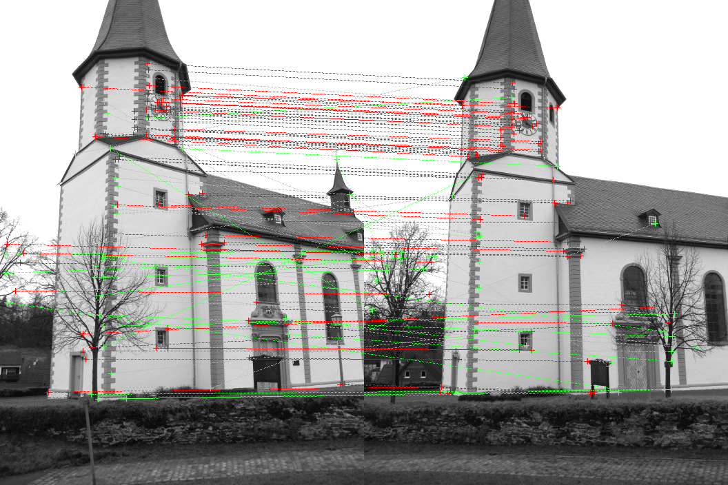
- Nearest neighbor + Lowe ratio test — accept a match only if the best descriptor distance is <~0.8× the second best. Simple, still everywhere.
- SuperGlue (Sarlin et al., 2020) — a graph neural network with self- and cross-attention over both images' keypoints, solving matching as partial assignment (Sinkhorn). Matches with context — a keypoint's neighbors help decide its correspondence — nearly doubling hard-condition localization recall when it appeared.
- LightGlue (Lindenberger et al., 2023) — SuperGlue accuracy at a fraction of the cost via early-exit on easy pairs and pruning of unmatchable points. The current default pairing: SuperPoint + LightGlue.
- Dense/detector-free: LoFTR (2021), RoMa (2024) — match at feature-map level with transformers, no keypoints at all; strongest on texture-poor scenes, at higher compute cost.
- Foundation 3D era: DUSt3R / MASt3R (2024) — transformers that regress 3D pointmaps (and matches) directly from image pairs without calibration, collapsing parts of the classic SfM pipeline into a single forward pass; MASt3R-SfM and successors are re-plumbing mapping itself.
07Alternative paradigms — and why the classic pipeline still wins
Absolute pose regression (APR)
PoseNet (Kendall et al., 2015): train a CNN to map image → 6-DoF pose directly. Elegant, fast, and — as Sattler et al. (2019) demonstrated — fundamentally limited: APR behaves like sophisticated image retrieval, interpolating among training poses rather than reasoning geometrically, so it fails to extrapolate to novel viewpoints and trails structure-based methods by an order of magnitude of accuracy. Verdict: historically important, production-irrelevant.
Scene coordinate regression (SCR)
Instead of regressing the pose, regress each pixel's 3D world coordinate, then solve PnP+RANSAC on the predictions — keeping the geometric engine but replacing the explicit descriptor map with a network that has memorized the scene. Line: SCoRe Forests (2013) → DSAC* (differentiable RANSAC, Brachmann & Rother) → ACE (2023): mapping a new scene in ~5 minutes with a 4 MB network, no depth needed, state-of-the-art in small-to-mid scenes → ACE-G (2025): query pre-training for generalization. The industrial home of this line is Niantic Spatial's research group (nianticspatial.com/research), which is betting on SCR and its descendants as the scalable map format; the same group's map-free relocalization (2022) goes further still — metric pose relative to a single reference photo, no map at all, the natural fit for pop-up AR at places nobody pre-scanned. Weaknesses: scale (city-level SCR remains open) and the retrain-on-change problem. For room-to-building scale with a fixed scene, SCR is the modern dark horse — an expert should know it well.
Implicit/neural maps
NeRF-based localization (iNeRF: invert a radiance field by gradient descent on photometric error) and 3D Gaussian Splatting-based relocalization replace the point cloud with a differentiable renderer: localize by "render-and-compare." Attractive properties: photorealistic maps double as content, analysis-by-synthesis handles viewpoint gracefully. Current status: compelling research, not yet at production robustness/scale; splatting's speed is rapidly closing the practicality gap, and hybrid schemes (feature-based init + render-and-compare refinement) are the likely landing zone.
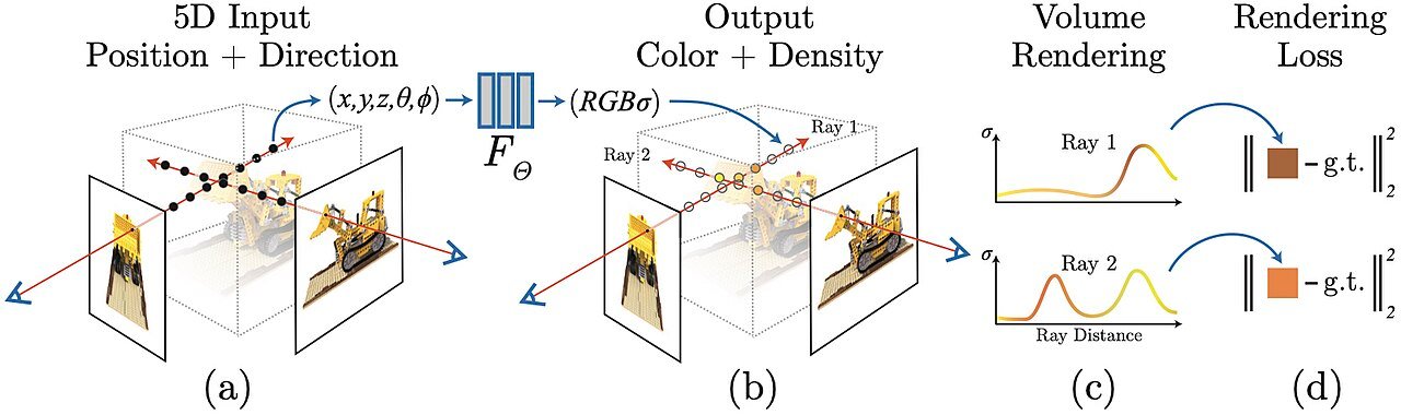
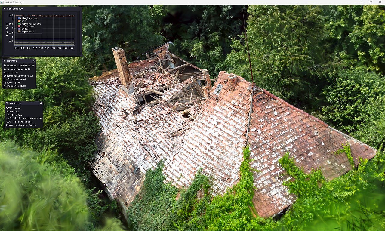
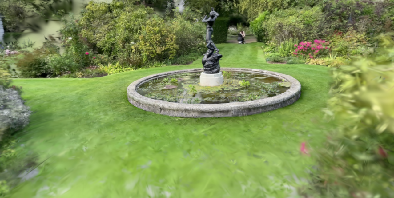
| Paradigm | Map | Accuracy | City scale | Update on change | Status |
|---|---|---|---|---|---|
| Structure-based (hloc) | SfM points + descriptors | cm–dm | Proven (planet) | Incremental re-map | Production default |
| APR (PoseNet line) | Network weights | m-level | No | Retrain | Superseded |
| SCR (ACE line) | Small network | cm | Open problem | Retrain (fast) | Strong niche |
| Neural rendering (NeRF/3DGS) | Radiance field / splats | cm (refinement) | Emerging | Partial re-fit | Research → hybrid |
08VPS + VIO — how production AR actually works
No shipping system calls the VPS every frame. The division of labor:
- On-device VIO (visual-inertial odometry — ARKit/ARCore's core): fuses camera tracking with IMU integration to deliver smooth 6-DoF motion at 30–60 Hz with low latency. Its flaw: the origin is arbitrary and the trajectory drifts (roughly ~1% of distance traveled, worse in feature-poor spaces), and it knows nothing of the world frame.
- VPS fixes — occasional (on session start, on demand, every few seconds-to-minutes, or when drift covariance grows): each fix is an absolute pose measurement in the world frame.
- Fusion — an extended Kalman filter or sliding-window pose-graph estimates the transform world ← odometry, treating VPS fixes as measurements with covariance and outlier gating (a bad fix must be rejectable — this is why honest confidence reporting in Section 5 matters). Corrections are applied gently (blended over frames) so virtual content never visibly teleports.
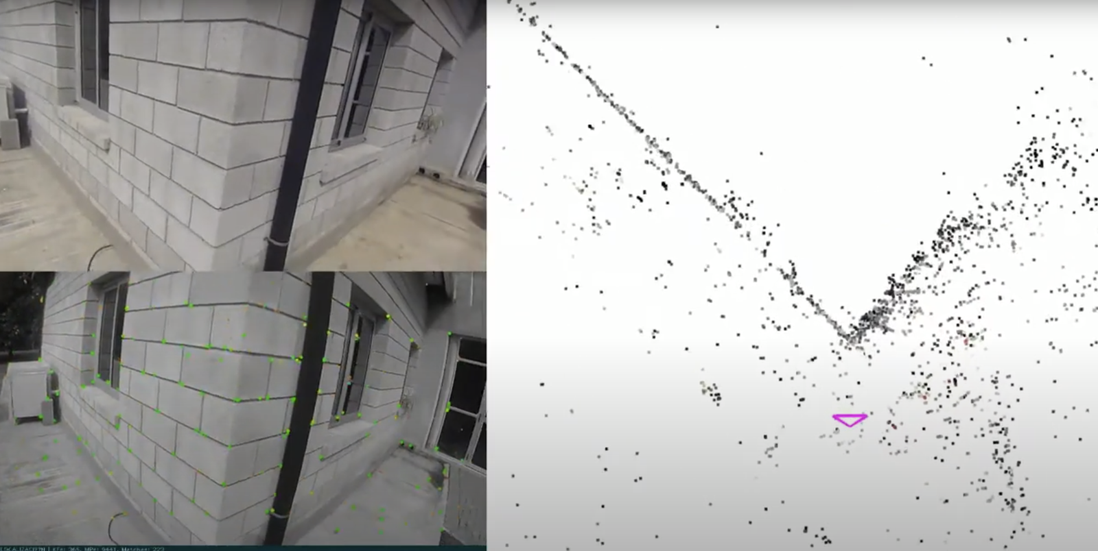
This architecture is why "VPS latency" of 200 ms is acceptable: the user experiences VIO's latency (~ms), while VPS merely re-anchors the frame occasionally. It is also the template for robotics: swap ARKit for a LiDAR-inertial odometry stack, keep the same global-fix logic.
Anchors — the content layer
An anchor is a named pose in the world frame to which content is attached ("the dragon stands at this plaza corner, facing the fountain"). Persistence (content survives sessions) and sharing (two users see the same dragon in the same spot) both reduce to: everyone localizes into the same map frame, anchors live in that frame. Cloud anchors, geospatial anchors, location anchors — every vendor's flavor is this one idea.
09Production systems survey
| System | Map source | Coverage model | Access | Notes |
|---|---|---|---|---|
| Google — ARCore Geospatial API (VPS since 2022) | Street View corpus (vehicle + Trekker imagery) | Outdoors, ~100+ countries wherever Street View exists | ARCore (Android/iOS/Unity), free tiers | The planet-scale reference. Geospatial anchors (lat/long/alt), Streetscape Geometry (building/terrain meshes), Scene Semantics. Accuracy commonly dm-level position, ~1° heading in well-mapped streetscapes. |
| Niantic — Lightship VPS (2022) | Crowdsourced: Pokémon GO/Ingress player scans, Scaniverse app, developer surveys | Point-of-interest–centric "VPS-activated locations" (1M+ claimed), city meshes in select areas | Lightship ARDK (Unity), 8th Wall (WebAR) | The crowdsourcing model at maximum. In 2025 Niantic sold its games business to Scopely and re-founded as Niantic Spatial around the map/VPS asset; announced "Large Geospatial Model" ambition (2024) — foundation-model positioning on top of the scan corpus. Its research arm publishes the strongest industrial localization line: ACE/ACE-G scene coordinate regression, map-free relocalization, cross-view splatting. |
| Apple — ARKit Location Anchors (ARGeoAnchor, iOS 14, 2020) | Apple Maps "Look Around" fleet imagery | Supported cities list (US, Tokyo, London, and growing) | ARKit (Swift), on Apple devices only | Tight OS integration, high-quality fleet data, conservative coverage. The same capability underlies AR walking directions in Apple Maps. |
| Immersal (acq. by Hexagon, 2021) | Developer/venue scans via SDK or drone | Per-venue: malls, airports, factories, stadiums | SDK (Unity, native), REST mapping API | The leading independent venue-VPS vendor; surveying-grade parent company; strong in industrial/enterprise deployments. |
| Snap — Custom Landmarkers | Creator phone scans + Snap's City Painter city meshes | Landmark/venue-centric | Lens Studio | Optimized for AR lenses at famous places; consumer-creative rather than infrastructure positioning. |
| Microsoft — Azure Spatial Anchors | Session feature maps (not a global map) | Per-space anchors | Retired November 2024 — instructive: cross-platform anchor service without a proprietary map corpus proved a weak moat. The map is the business. | |
| Others | MultiSet AI (commercial venue-scan VPS reaching consumer smart glasses, phones, and robots), Sturfee (satellite-imagery-derived VPS), Naver Labs (Korea, indoor+outdoor, strong research group and the Kapture toolset), Meta (research: Project Aria glasses corpora, LSD/Aria datasets feeding future wearable localization), automotive lane-level relocalization (Mobileye REM crowdsourced maps — VPS logic at highway scale). | |||

10The hard problems
1 · Long-term appearance change
Day↔night, summer↔winter, dry↔snow, renovation. The map was photographed under one condition; the query arrives under another. This is the canonical research problem — the Aachen Day-Night, RobotCar Seasons, and CMU Seasons benchmarks (Section 11) exist precisely to measure it. Mitigations: condition-robust learned features and retrieval (the main line of progress), mapping multiple conditions, semantic filtering (match on buildings, ignore vegetation — geometry stable, appearance volatile), and appearance-transfer augmentation at training time.
2 · Dynamic and ambiguous scenes
Crowds, vehicles, and merchandise occlude and pollute; identical corridors, glass, and chain-store facades alias. Mitigations: semantic masking of transient classes at both mapping and query time, multi-frame queries, position priors, and RANSAC's inherent outlier tolerance. Glass and mirrors remain genuinely unsolved for feature-based methods.
3 · Scale and freshness economics
Mapping the world once is capex; keeping it fresh is opex forever. The engineering answers: change detection (localization failure rates per tile are themselves the staleness signal), incremental map updates (register new imagery into the existing model rather than rebuilding), and crowdsourcing the refresh loop (Section 9's strategic read). Map compression (Section 4) governs serving cost.
4 · Privacy — both directions
- Map privacy: SfM point clouds with descriptors are not anonymous geometry — Pittaluga et al. (2019) showed recognizable images can be reconstructed by inverting descriptors. Proposed defenses: lifting points to lines (Speciale et al., 2019) — later shown partially attackable (Chelani et al., 2021) — descriptor-free geometric matching (GoMatch line), and splitting sensitive computation between device and server. An active cat-and-mouse literature.
- Query privacy: every localization uploads what the user's camera sees, tied to a precise pose. Production mitigations: on-device feature extraction (send descriptors, not pixels), ephemeral processing commitments, and on-device localization against downloaded map tiles (the strongest answer, adopted for sensitive venues).
5 · Integrity and spoofing
Rarely discussed, increasingly relevant as robots act on VPS output: a printed poster of a known facade is the visual analog of GPS spoofing. Defenses mirror GNSS thinking — multi-frame consistency with ego-motion, cross-checking against VIO and coarse radio position, and geometric liveness (a flat poster fails parallax checks across two frames).
11Benchmarks, metrics, and how to read a leaderboard
The metric
Visual localization is scored as recall at pose-error thresholds: the percentage of query images localized within both a position and an orientation bound. The community-standard triple (from the Long-Term Visual Localization benchmark, visuallocalization.net):
Read all three together: the first tells you AR-grade precision, the last tells you gross failure rate. A method with great (0.25 m) recall but poor (5 m) recall fails catastrophically when it fails — often worse in production than a method that degrades gracefully.
The benchmark canon
| Benchmark | Setting | What it stresses |
|---|---|---|
| Aachen Day-Night (v1.1) | European old town; day map, day+night queries | The day→night appearance gap; the single most-cited outdoor benchmark |
| RobotCar Seasons | Same Oxford route driven ~year-round | Seasonal/weather change from a vehicle; rain, dusk, snow, sun |
| Extended CMU Seasons | Pittsburgh suburbs across seasons | Vegetation change — foliage is the enemy |
| InLoc | University buildings, RGB-D map | Indoor: texture-poor walls, repetitive structure, furniture churn |
| 7-Scenes / 12-Scenes | Small RGB-D rooms | The SCR/APR playground; saturated for structure-based methods |
| Cambridge Landmarks | Five outdoor landmarks | Historic APR benchmark; still used for method comparison |
Reading a leaderboard like an expert
- Check which stage differs between entries — many "new SOTA" rows are the same hloc skeleton with one component swapped. Attribute the gain to the component, not the brand.
- Check compute honesty: dense matchers (RoMa-class) buy recall with 10–100× matching cost; a production system cares about recall per millisecond per dollar.
- Check the night column first on Aachen — day columns have been near-saturated for years; hard conditions are where methods actually separate.
- Distrust single-benchmark wins; the canonical methods (SuperPoint+LightGlue+hloc) win by being uniformly strong everywhere, which is what deployment requires.
12Build your own VPS — the practical recipe
A venue-scale VPS (shop, mall, campus, factory) is a weekend-to-week project on open source. The reference stack:
| Component | Tool | Role |
|---|---|---|
| Pipeline framework | hloc (github: cvg/Hierarchical-Localization) | Glues everything below into mapping + localization scripts |
| SfM engine | COLMAP (+ pycolmap) | Reconstruction, triangulation, bundle adjustment, PnP |
| Local features | SuperPoint (or ALIKED/XFeat for lighter) | Keypoints + descriptors |
| Matcher | LightGlue | Robust correspondence |
| Retrieval | NetVLAD (or SALAD/DINOv2-based for harder conditions) | Top-k map image shortlist |
| Dataset plumbing | Kapture (Naver) — optional | Standardized sensor/trajectory data format |
The recipe
# 1 · CAPTURE — walk the venue; video → frames (1–2 fps), or 200–2000 photos.
#     Overlap generously; revisit from opposing directions; capture at the
#     times-of-day you expect queries. Loop closures matter more than count.

# 2 · MAP — hloc: extract features, match pairs, run COLMAP SfM
extract_features (superpoint)  →  pairs_from_retrieval (netvlad, top-40)
→  match_features (lightglue)  →  reconstruction (COLMAP)
# Output: sparse model (cameras.bin, images.bin, points3D.bin) + feature DB

# 3 · GEOREFERENCE — align the model to your venue frame:
#     mark 3+ surveyed control points in images, solve the 7-DoF similarity
#     (COLMAP model_aligner), or accept the arbitrary frame for AR-only use.

# 4 · LOCALIZE — per query image:
retrieval top-k  →  match query↔retrieved  →  lift to 2D–3D
→  pycolmap absolute_pose_estimation (P3P+RANSAC+refine)
# Returns: pose, num_inliers  →  accept if inliers ≥ ~50 (tune on your venue)

# 5 · SERVE — wrap step 4 in a service; client sends frame + intrinsics
#     (and gravity if available), receives pose + confidence.
The latency budget (single GPU server, 1080p query)
| Stage | Typical cost | Levers |
|---|---|---|
| Feature extraction (query) | 10–30 ms | Resolution, lighter detector, on-device extraction |
| Retrieval | 1–10 ms | ANN index (FAISS), tile pre-filter by radio prior |
| Matching (k images) | 20–150 ms | k, LightGlue early-exit, covisibility clustering |
| PnP + RANSAC + refine | 2–15 ms | Gravity prior, MAGSAC++, inlier threshold |
| Total (server-side) | ~50–200 ms | Well inside the VIO-fusion architecture's tolerance |
Judgment calls that decide success
- Capture discipline beats algorithm choice. A mediocre pipeline on thorough, multi-condition capture outperforms SOTA on a thin single-pass scan. Budget 70% of effort here.
- Set the acceptance threshold empirically. Walk the venue with ground truth (or self-consistency checks: sequential queries must yield VIO-consistent poses) and choose the inlier cutoff that kills every wrong fix. False fixes are the product-killer.
- Plan the refresh loop on day one. Decide what triggers re-mapping (failure-rate per zone), and make map updates incremental (register new images into the existing model — hloc/COLMAP support this) rather than rebuild-the-world.
- On-device vs server: venue maps of a few hundred MB can ship to the device (privacy, latency, offline); city maps cannot. The hybrid — device extracts features, server matches — is the common production compromise.
13Applications and the business lens
- AR navigation & persistent content — airport/mall/hospital wayfinding with arrows painted on the floor through the camera; city-scale AR layers (Google Maps Live View is VPS-powered). The flagship consumer application.
- Robotics last-meter — warehouse AMRs, delivery robots, and service robots use VPS-style relocalization to recover pose after kidnap/restart and to anchor to semantic infrastructure ("dock #7"), where GPS is absent and wheel+LiDAR odometry drifts.
- Drones in GPS-denied/degraded settings — indoor inspection, under-bridge survey, urban canyons; and as GPS-jamming resilience: terrain/landmark-relative visual navigation is the civilian cousin of military visual-aided inertial navigation.
- Industrial digital twins — technician points a tablet at a pump; the twin overlays torque specs and maintenance history. VPS is the registration layer between the twin and reality (Immersal/Hexagon's core market).
- Automotive lane-level localization — camera-relocalization against crowdsourced sparse maps (Mobileye REM) delivers lane-keeping-grade position where GNSS cannot.
- Accessibility — precise position + heading enables turn-by-turn guidance for blind and low-vision users indoors, a domain where meter-level error is the difference between usable and useless.
The economics in three sentences
Mapping is a fixed cost per venue/city; localization is a near-zero marginal cost per query — classic infrastructure economics with winner-take-most dynamics per geography. The moat is never the algorithm (open source is within a few percent of any proprietary stack); it is the imagery corpus and its refresh loop. Consequently the viable entries are: own a fleet (Google/Apple), own a crowd (Niantic/Mobileye), own the venue relationship (Immersal-style enterprise), or serve where giants won't — private facilities that will never let a fleet inside and want on-premises maps for confidentiality.
14Expert self-test
Fifteen questions. An expert answers ~13 without looking. Answers fold open.
1 · Why does a VPS provide orientation "for free" while GPS cannot?
2 · Why is monocular SfM scale-ambiguous, and name three ways scale is injected.
3 · Why retrieval-then-match instead of matching against the whole map?
4 · What does the RANSAC iteration formula N = log(1−p)/log(1−wˢ) imply about minimal solvers?
5 · Where is the camera center in world coordinates, given pose [R|t]?
6 · Why did SuperGlue outperform ratio-test matching so dramatically?
7 · Why is absolute pose regression (PoseNet-class) not used in production VPS?
8 · Your night-time recall collapses. Which stage do you check first and how?
9 · Why does a phone's gravity estimate materially improve pose solving?
10 · What is the covisibility graph and why does localization use it?
11 · Why is a confidently wrong pose worse than no pose in production?
12 · The privacy attack on SfM maps, and the defense arc?
13 · Why did Azure Spatial Anchors die while Google/Niantic VPS thrived?
14 · When would you pick scene coordinate regression (ACE) over the hloc stack?
15 · Sketch the full production loop from camera frame to stable AR content.
15Glossary
- 6-DoF pose
- Position (x,y,z) + orientation (roll,pitch,yaw); mathematically [R|t], R ∈ SO(3).
- Anchor
- A named pose in the map/world frame to which virtual content or semantics attach.
- Bundle adjustment (BA)
- Joint nonlinear least-squares refinement of all poses and 3D points minimizing total reprojection error.
- Covisibility graph
- Graph recording which map points are observed together from which images; used for clustering and consistency.
- Descriptor
- A vector summarizing local appearance around a keypoint (local, e.g. SuperPoint 256-D) or of a whole image (global, e.g. NetVLAD) for matching/retrieval.
- Epipolar geometry
- The two-view constraint (essential/fundamental matrix) relating corresponding points; the verification tool of pairwise matching.
- Extrinsics / intrinsics
- Pose [R|t] (world→camera) / internal projection parameters K plus lens distortion.
- Georegistration
- 7-DoF similarity alignment (R, t, scale) of a reconstruction to an Earth-fixed frame.
- hloc
- Hierarchical Localization — the retrieval → match → PnP reference architecture and its open-source implementation.
- Inlier
- A correspondence consistent with the estimated model within threshold; inlier count ≈ pose confidence.
- Keyframe
- A selected representative frame retained in a map or SLAM graph.
- Perceptual aliasing
- Distinct places that look alike (corridors, chain stores), inducing confident wrong retrieval/matches.
- PnP / P3P
- Perspective-n-Point: pose from n 2D–3D correspondences with known intrinsics; P3P is the 3-point minimal case.
- RANSAC
- Random Sample Consensus — robust estimation by minimal-sample hypothesize-and-verify voting.
- Relocalization
- Recovering pose in an existing map after tracking loss or at session start — the VPS operation, viewed from SLAM.
- Reprojection error
- Pixel distance between a projected 3D point and its observed feature; the universal objective.
- Retrieval (VPR)
- Visual place recognition: finding which map images/places match a query, via global descriptors.
- Scene coordinate regression
- Regressing per-pixel 3D world coordinates with a scene-specific network, then PnP (DSAC*, ACE).
- SfM
- Structure from Motion — joint recovery of 3D structure and camera poses from image collections (COLMAP).
- SLAM / VIO
- Simultaneous Localization and Mapping / Visual-Inertial Odometry — online tracking (+mapping) in unknown space; VIO is the camera+IMU odometry core of ARKit/ARCore.
- Triangulation
- Intersecting rays from ≥2 posed views to place a 3D point.
- WiFi CSI
- Channel State Information — per-subcarrier amplitude/phase of the WiFi channel, a multipath fingerprint of a space; enables device-free sensing (presence, gesture, fall, respiration) and sub-meter radio positioning (IEEE 802.11bf).
16Reading list — the canon, in reading order
- 1981Fischler & Bolles — RANSAC ("Random Sample Consensus") — robust estimation, born from camera pose.
- 2004Lowe — SIFT ("Distinctive Image Features from Scale-Invariant Keypoints").
- 2004Hartley & Zisserman — Multiple View Geometry in Computer Vision — the field's textbook; chapters on projection, two-view geometry, and BA are the mathematical bedrock.
- 2009Lepetit et al. — EPnP — O(n) PnP.
- 2015Kendall et al. — PoseNet — absolute pose regression (read with its 2019 refutation, below).
- 2016Schönberger & Frahm — COLMAP ("Structure-from-Motion Revisited").
- 2016Arandjelović et al. — NetVLAD — learned place recognition.
- 2018DeTone et al. — SuperPoint — self-supervised keypoints.
- 2018Sattler et al. — Benchmarking 6DOF Outdoor Visual Localization in Changing Conditions — Aachen/RobotCar/CMU benchmark paper.
- 2019Sarlin et al. — From Coarse to Fine: Robust Hierarchical Localization at Large Scale — the hloc paper; the modern VPS blueprint.
- 2019Sattler et al. — Understanding the Limitations of CNN-based Absolute Camera Pose Regression — why APR ≈ retrieval.
- 2019Pittaluga et al. — Revealing Scenes by Inverting Structure from Motion Reconstructions — the privacy attack.
- 2020Sarlin et al. — SuperGlue — attention-based matching.
- 2021Sun et al. — LoFTR — detector-free transformer matching.
- 2023Lindenberger et al. — LightGlue — fast adaptive matching.
- 2022Arnold et al. — Map-free Visual Relocalization — metric pose from a single reference image, no map at all.
- 2023Brachmann et al. — ACE ("Accelerated Coordinate Encoding") — 5-minute scene coordinate mapping.
- 2023Keetha et al. — AnyLoc — foundation-model (DINOv2) place recognition.
- 2024Wang et al. / Leroy et al. — DUSt3R / MASt3R — pointmap regression; the foundation-model turn in 3D matching and SfM.
Live resources: visuallocalization.net (benchmark + leaderboard) · github.com/cvg/Hierarchical-Localization (hloc) · colmap.github.io (COLMAP docs) · Image Matching Challenge (CVPR, annual) for the state of matching. Watching: YouTube @bilawalsidhu — Bilawal Sidhu, formerly the Google product lead behind 3D Maps / ARCore Geospatial (the Google VPS of Section 9), now a 2M-subscriber explainer of reality capture, Gaussian splatting, and spatial intelligence; the moving-picture companion to this report.
17Plain speak — the whole report, retold simply
1 · What it is
A VPS tells a camera exactly where it is and which way it is pointing, by recognizing what it sees against a prepared 3D memory of the place. GPS guesses your dot from satellites — meters off, no idea which way you face, dead indoors. A VPS is accurate to centimeters, knows your facing, and works indoors — but only where someone has already built the map. Hold one idea above all: it is not a sensor, it is recognition against a map. One cousin worth knowing: WiFi CSI — the router's radio echo of a room. It can sense people moving even through walls, but it can never deliver the precise position-plus-facing a camera can; the two work best together.
2 · The geometry
A camera is a machine that drops 3D points onto a flat sensor. If you know which 3D points landed on which pixels, there is only one place the camera can be standing — and finding that place is the whole game. "Reprojection error" is simply how far off the landing predictions are for a guessed position; every algorithm in the field works to make that number small. Three good point-to-pixel pairs already give a candidate answer. And because many pairs are wrong, the answer is chosen by a voting trick: try many small random samples, keep the answer the most pairs agree with. Matching proposes; voting disposes.
3 · The two phases
Build the map once, slowly and expensively: photograph everything, compute a 3D model. Then answer questions forever, fast and cheaply: recognize, match, solve. It is the same shape as a search engine — crawl offline, serve online — and just like search, whoever owns the index owns the business.
4 · Making the map
Take many overlapping photos. Software finds the same small details across different photos and works out, simultaneously, where every photo was taken and where every detail sits in 3D. A final clean-up pass spreads the small errors evenly so nothing accumulates. One catch: photos alone cannot tell true size — a dollhouse and a house photograph identically — so real-world scale must come from outside: GPS, measured reference points, or the phone's motion sensors. The finished map is a cloud of 3D dots, each remembering what it looks like. That memory is what queries match against.
5 · Answering a query
Three shrinking questions. Which part of town? — a fast whole-image similarity search picks a handful of map photos. Which details match? — compare the small features between the query and those photos. Where must the camera stand so that everything lines up? — geometry gives the spot and the facing. Then the honesty meter: count how many matches truly agree with the answer. If too few agree, say "no fix." A confident wrong answer is the worst thing this system can produce, because everything downstream trusts it.
6 · Recognizing details
A "feature" is a small recognizable detail — a corner, an edge, a mark. For twenty years, hand-written math decided what counts as a detail and whether two look alike. Today, neural networks learn both — and they read the whole image for context before deciding any single match. Each generation of this technology survives worse conditions than the last: night, rain, snow, and big changes of viewpoint.
7 · The rival ideas
Three challengers have tried to replace the classic recipe. Let a network look at a photo and guess the position outright — it turned out to memorize rather than measure, and fails away from its training shots. Let a network memorize one scene's 3D shape so every pixel can name its 3D point — this genuinely works for a single building, but must be retrained when the scene changes and does not scale to cities. Make the map photorealistic and search inside it like a rendering — promising and young. At city scale, the classic recipe still beats all three.
8 · Living with the phone's own tracking
Phones already track their own motion smoothly, using the camera and motion sensors together — but like a step-counter, they slowly wander off course. The VPS plays the role of the trail sign: every so often, look up, check, correct. The user experiences only the smooth track; corrections are blended in so nothing visibly jumps. "Anchors" are named spots saved in the shared map where content lives — which is why two people's phones can show the same virtual object standing on the same real corner.
9 · Who runs the big ones
Google built its VPS from Street View — it covers much of the world's streets. Niantic built its map from millions of players' phone scans — strongest at interesting places. Apple flew and drove its own fleet — select cities, tightly integrated. Immersal walks your building for you — venues and factories. Microsoft ran an anchor service with no camera corpus of its own, and it is the one that shut down. The lesson in one line: the map is the moat, not the math.
10 · What is still hard
The map is a photograph of the past; every query is the present. Night, snow, and renovations break the resemblance. Identical corridors and repeated storefronts fool the recognizer. Keeping maps fresh costs money forever. Privacy cuts both ways: map data can be reverse-engineered back into images of the place, and every query shows a server what your camera sees. And the system can in principle be spoofed with a printed picture of a place — though a poster is flat, and flat things fail the parallax check when the camera moves.
11 · Keeping score
The standard exam: out of 100 query photos, how many were placed within 25 centimeters and 2 degrees of the truth? Also watch the loose 5-meter score — when the system misses, it should miss near, not teleport across town. And always read the night-time results first; the daytime exam was solved years ago.
12 · Build one yourself
One person, one phone, a weekend, free software. Film the venue walking slowly, from both directions, at the times of day you care about. Free tools turn the footage into a 3D map. A small program answers queries: similarity search, detail matching, geometry. Spend your effort where it counts — thorough filming beats clever algorithms — and set the "no fix" threshold strictly, so a wrong answer never escapes. Decide on day one how you will re-map when the venue changes, because it will.
13 · Where the money is
Anywhere someone or something needs "exactly where am I, facing which way" and GPS cannot answer: navigation arrows painted through the camera in malls, airports, and hospitals; robots finding their dock; drones where GPS is absent or jammed; a factory tablet that recognizes the machine it is pointed at; cars holding their lane. The cost model: expensive to map once, nearly free per query after — value concentrated exactly where GPS is blind.
14–16 · The wrap-up, plain
Test yourself with five one-breath questions: why does a VPS know your facing while GPS never can; why can photos alone not tell true size; why does matching against the whole map at once fail; why is "no fix" better than a wrong fix; why did the service without its own cameras die? Answer those cleanly and Section 14's full exam will go well. The vocabulary reduces to five items: pose = position + facing; features = recognizable details; structure-from-motion = photos in, 3D out; PnP + RANSAC = geometry + voting; hloc = the standard recipe wiring it all together. And if you read only four papers, read them in this order: SIFT, COLMAP, hloc, SuperGlue — the detail, the map, the recipe, the matcher.
18The future — a futurist's map
Forecasting discipline, stated up front: three horizons, each claim tagged by confidence — HIGH mechanism already visible and funded, MED trajectory clear but timing uncertain, SPEC plausible discontinuity. Reasoning from mechanisms, not enthusiasm.
Near term, to ~2029 — consolidation
- HIGH Foundation models eat the pipeline. MASt3R-class pointmap transformers keep collapsing detect–describe–match–reconstruct into forward passes. The hloc skeleton survives as scaffolding, but its stages become heads of one model; "which feature, which matcher" stops being a decision anyone makes.
- HIGH Splat-native maps. 3D Gaussian Splatting matures into a mainstream map format — one asset that is simultaneously the localization substrate, the rendering, and the content. The map you localize against becomes the map you look at.
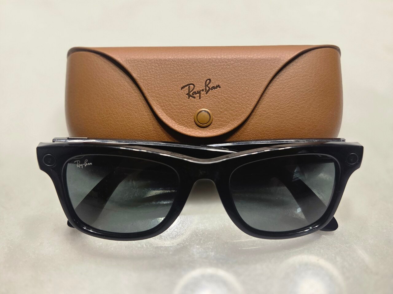
- HIGH Glasses make queries continuous. Ray-Ban-class wearables turn VPS from an episodic call into an always-available service; localization moves from "open the app and scan" to ambient. The §13 case study was the preview.
- HIGH Radio sensing ships. 802.11bf-era access points make WiFi CSI sensing a checkbox feature; indoor stacks default to radio-prior + visual-fix fusion. Presence becomes free; pose stays visual.
- MED Mapping flywheels formalize. Scan-to-earn, mapping-as-byproduct-of-play, fleet-as-mapper (the Niantic and Mobileye patterns) become explicit business models with contracts and marketplaces rather than happy accidents.
Why this horizon is safe to bet on. Every claim above has its mechanism already shipping: the pointmap models exist and win benchmarks, splat tooling is in consumer apps, the glasses are on faces, and 802.11bf is the standards body confirming what labs proved a decade ago. When a capability moves from paper to standard to checkbox, the remaining uncertainty is packaging, not physics. The practical instruction for a builder: keep the classic modular stack (its interfaces are where the coming model boundaries will land), and accumulate capture assets now — every scan taken today is compatible with every future map format, because all of them are trained from imagery.
Mid term, ~2029–2033 — the world-model era
- MED Large Geospatial Models arrive. The database lookup becomes a model query: one foundation model holds an implicit, compressed memory of much of the mapped world. Map-free relocalization and LGMs converge on the same promise — a metric pose from one photograph, almost anywhere. The visuallocalization.net leaderboard becomes a model benchmark.
- MED Neural maps displace point clouds. The canonical map format stops being points-plus-descriptors and becomes learned weights or splats. The §10 privacy attack surface changes shape entirely — descriptor inversion dies, model inversion is born, and the attack/defense literature restarts.
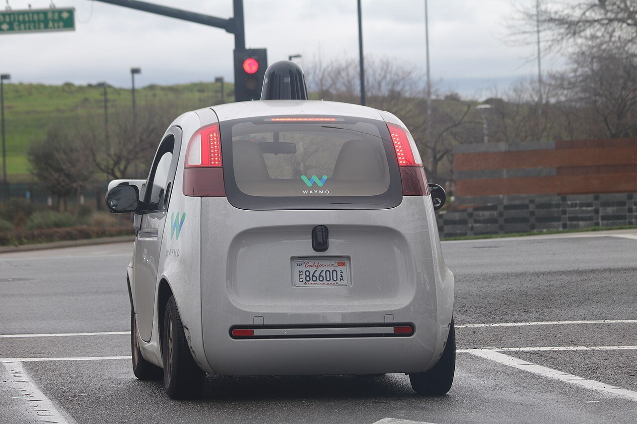
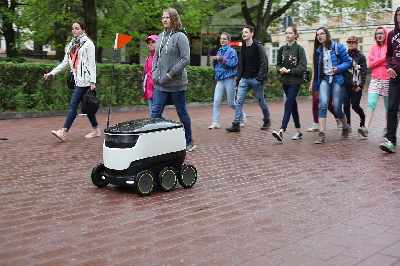
- MED Robots become the majority user. Humanoids, AMRs, drones, and delivery fleets issue more localization queries than humans. Maps re-optimize for machine consumption: semantics, affordances, and traversability first; photorealism becomes a human-facing view, not the substance.
- MED Anchors become civic infrastructure. Persistent shared AR forces the unglamorous questions: who may anchor content at a place, who owns the map of a private building, which jurisdiction's rules bind a world-readable coordinate. Expect "map sovereignty" contracts and the first serious litigation.
- SPEC Integrity becomes regulated. Once robots act on visual fixes, visual spoofing graduates from curiosity to attack class; safety-critical domains (automotive, aviation, defense) get certified-integrity localization the way GNSS got RAIM.
Why this horizon rhymes with search. The web went through exactly this transition: first an index you queried (retrieve, then read), then models that had internalized the corpus and answered directly. Maps are next, and the same consequences follow. Coverage moats weaken — a model that generalizes needs less bespoke per-place data — while freshness and trust moats strengthen, because a model's memory of the world ages just like an index does but is harder to audit. The second repricing force is demand: a delivery fleet queries localization thousands of times per vehicle per day, so the customer of record shifts from a person opening an app to a machine that never stops asking. Infrastructure gets rebuilt for whoever pays most often.
Far term, ~2033–2040 — ambient spatial intelligence
- MED The world becomes self-mapping. Every camera-bearing device is a mapping sortie; freshness approaches real time; the map converges on a live digital twin of the inhabited world — the "mirrorworld" thesis, arriving as infrastructure rather than spectacle.
- MED Positioning dissolves as a category. Pose becomes ambient metadata the OS provides, like the clock. "VPS vendor" sounds as dated as "GPS app vendor" does today; the value migrates up-stack to what pose enables — anchored content, spatial agents, machine action.
- SPEC Sensor totalism. Vision + CSI + UWB + event cameras + chip-scale inertial fuse so deeply that no single sensor is load-bearing; positioning degrades gracefully everywhere, including darkness, smoke, and jamming.
- MED The privacy fork decides geography. Both endpoints are technically feasible: maps ship to the device and nothing leaves it, or everything resolves in clouds that see every query. Jurisdictions will fork on this line, and the fork — not accuracy — will decide which architectures win which markets.
Why "ambient" is the destination. There is a clean historical precedent: precise time. Once a scarce service — marine chronometers, radio time signals, a product category — time is now free metadata that every device carries and no user thinks about, yet an entire hidden infrastructure (atomic clocks, NTP, GNSS timing) keeps it running. Position is on the same path: the infrastructure grows more elaborate while the experience disappears. When that happens, the visible economy moves entirely to what pose enables, and the invisible economy — who operates the world's memory, under whose rules — becomes one of the quiet strategic assets of the century.
What to adopt today — the practitioner's radar
A technology radar for anyone building spatial capability now, chosen by three tests: is it mature enough to trust, cheap enough to deploy this quarter, and does using it compound — leaving you with data, infrastructure, or skill that every future generation of the stack will still consume?
| Tier | Technology | What it gives you today | Why alongside VPS + CSI |
|---|---|---|---|
| ADOPT NOW | VIO (ARKit / ARCore) | Free, smooth 6-DoF tracking on every phone in your building | The local layer every VPS fix anchors; costs nothing, required regardless of future stack |
| 3D capture & splatting (Scaniverse, Polycam, RealityCapture) | Photoreal scans of your venues from a phone, today | Scans are the compounding asset — compatible with every current and future map format, since all are trained from imagery. Start the archive now | |
| Fiducials (AprilTag / ArUco / QR) | Millimeter-grade anchors and ground truth for cents per printed marker | Instant accuracy where maps are thin; calibration and truth data for evaluating your VPS honestly | |
| UWB (in flagship phones + cheap tags) | 10–30 cm radio ranging, indoors, through light occlusion | The precision radio complement: CSI senses presence, UWB pins distance, VPS delivers full pose | |
| WiFi RTT (802.11mc) + BLE beacons | Meter-class indoor position from existing or trivially-added infrastructure | The coarse prior that feeds the VPS funnel (§5) — better tiles, instant floor disambiguation | |
| Open localization stack (COLMAP, hloc, SuperPoint, LightGlue) | Production-grade mapping + localization, free | Owning the pipeline in-house builds the judgment every later buy-vs-build decision needs | |
| PILOT | Smart glasses (Ray-Ban class) | Hands-free capture and continuous queries | The §13 case study hardware — learn its constraints before it becomes the default client |
| WiFi CSI sensing rigs (ESP32, pre-802.11bf) | Device-free presence, flow, and fall detection for a few dollars a node | Cheap operational analytics now; positions you for 802.11bf silicon on arrival | |
| Phone LiDAR scanning (iPhone/iPad Pro) | Metric depth for true-scale models and ground truth | Fixes monocular SfM's scale blindness (§4) at consumer cost | |
| MASt3R-class & map-free models | Pose estimates with little or no pre-built map | Evaluate now on your hardest sites — this is the boundary the field is moving toward | |
| WATCH | Large Geospatial Models | Not yet purchasable; when pose-from-one-photo-anywhere ships, re-derive your map strategy that quarter | |
| Event cameras / neuromorphic | Microsecond low-power sensing — the always-on-glasses sensor; toolchains still research-grade | ||
| Chip-scale quantum / photonic INS | The architecture inverter (drift-free dead reckoning); nothing to deploy, everything to track | ||
| LEO PNT constellations | Would repair GNSS's urban weakness from orbit; watch coverage announcements, not demos | ||
The adoption logic, stated once: the ADOPT tier is entirely things that leave permanent residue — scan archives, installed radio, anchored markers, in-house skill. Even if every model in this report is replaced (it will be), that residue transfers. The PILOT tier is tuition: small deployments whose real product is your team's judgment about a coming device class. The WATCH tier is deliberately not built upon — each entry is an architecture-breaker, and the correct posture toward architecture-breakers is a tripwire, not an investment.
Wildcards — discontinuities worth watching
- SPEC Chip-scale quantum/photonic inertial navigation good enough to hold drift-free pose for hours would invert the architecture: VPS becomes an occasional calibrator, not a tracker.
- SPEC LEO PNT constellations (dedicated low-orbit positioning) repairing GNSS's urban and indoor-adjacent weaknesses would compress outdoor VPS value toward orientation and semantics.
- SPEC Event cameras + neuromorphic compute: microsecond-latency, milliwatt localization — the natural sensor for always-on glasses, and a reset of the feature-extraction literature.
- SPEC Generative reality attacks. When scenes can be synthesized at will, place recognition needs provenance: proving a view is the real place, now becomes its own discipline — reality authentication as the last mile of localization.
The futurist's razors
Five principles that survive any particular timeline. Bet on flywheels, not features — every durable winner in Section 9 owns a self-refreshing capture loop, and that logic only strengthens. The map is the moat until world models make maps liquid — the moment a foundation model localizes anywhere from one photo, moat value migrates from coverage to freshness, semantics, and trust. Watch robot fleets, not phone apps — machine demand is the real volume signal for this infrastructure. Privacy architecture is strategy, not compliance — where resolution happens (device or cloud) will decide market access more than benchmark scores. And when pose becomes free, the value moves to what you do with it — the anchors, the semantics, the actions taken in the world; positioning was never the product, the positioned world is.